Clustered Data and the Sampling Budget

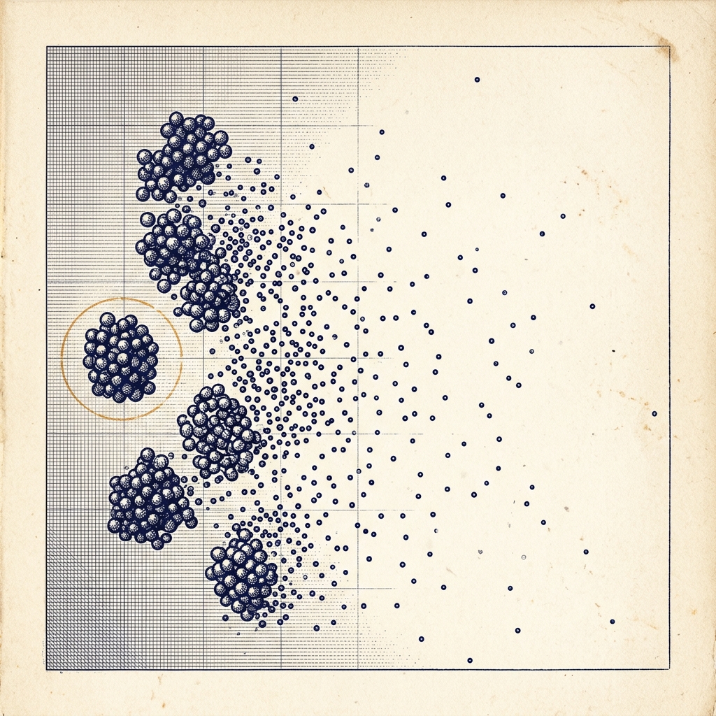
One Bad Tool Call, Ten Bad Rows

Your agent eval grades 100 conversations, 10 turns each: 1,000 graded rows. The pass rate comes in at 70%, and the naive 95% confidence interval is

Tight. Shippable. Also wrong.

Turns within a conversation sink or swim together. One bad tool call on turn 2 poisons the next nine rows; a conversation that starts clean tends to stay clean. If the intraclass correlation is $\rho = 0.5$—half of the outcome variance lives between conversations—the design effect is

The effective sample size is $1000 / 5.5 \approx 182$, and the honest interval is $\pm\, 2.8 \times \sqrt{5.5} \approx \pm\, 6.7$ pp. Your error bars were 2.3× too tight, and nobody lied. The rows just weren't independent.

This is the third post in the Error Bars for Evals strand. The first put a confidence interval on a single score; the second compared two models on the same questions. This one asks what happens when your rows arrive in clumps—and where the next thousand dollars of eval budget should go.

The Whole Idea in One Formula

Everything runs through the intraclass correlation $\rho$: the share of outcome variance that lives between clusters rather than within them. $\rho = 0$ means knowing one turn's outcome tells you nothing about its siblings. $\rho = 1$ means a conversation passes or fails as a unit and the turns are photocopies.

Given $\rho$ and a common cluster size $m$, Kish's design effect says how much clustering inflates the variance of your pass rate:

Two corollaries do all the practical work:

Anchor the formula at its edges:

• $m = 1$ → no penalty, ever. One row per cluster is just an independent sample, whatever $\rho$ is.
• $\rho = 0$ → no penalty, ever. Independent rows are independent rows, however you bundle them.
• The penalty is depth × stickiness. It grows with how deep each cluster goes ($m - 1$) multiplied by how much the rows inside it move together ($\rho$). Neither alone hurts you; the product does.

The Budget Identity

The second big idea decides how to spend. Fix a budget of $n = K \cdot m$ rows—$K$ clusters, $m$ rows each—and expand the variance of the pooled pass rate:

Read it out loud. The first term has the full budget $Km$ in its denominator: any spending shrinks it, depth or breadth alike. The second term has only $K$. There is no $m$ in it anywhere—no amount of extra depth touches it. Once $\rho$ is meaningful, that second term becomes the floor under your precision, and deeper clusters stop buying you anything. Only more clusters do.

A Worked Example

Take the eval from the hook: $K = 100$ conversations, $m = 10$ turns, and a pilot estimate of $\rho = 0.5$. The same five steps appear in the practice exercise below.

Step 1 — count the rows. $n = K \cdot m = 100 \times 10 = 1{,}000$. This is the $n$ the dashboard reports.

Step 2 — the design effect. $\mathrm{DEFF} = 1 + (10 - 1) \times 0.5 = 5.5$. Each conversation's ten turns carry the information of roughly two independent rows, not ten.

Step 3 — effective sample size. $n_{\mathrm{eff}} = 1000 / 5.5 \approx 182$. A thousand rows doing the work of 182.

Step 4 — the bar-widening factor. $\sqrt{5.5} \approx 2.35$. Every naive standard error in the report needs to stretch by 2.35× before you believe it.

Step 5 — spend the next budget. Leadership doubles your spend to 2,000 rows. Two ways to use it:

Same money. Doubling depth bought almost nothing (182 → 190 effective samples); doubling clusters doubled the work done (182 → 364). The budget identity said this would happen: option (b) poured its entire raise into the term that $m$ can't reach.

Where Clusters Hide in LLM Evals

Conversations are the obvious case. They are not the only one.

Miller's "Adding Error Bars to Evals" treats exactly this structure—question groups drawn from a shared context—and recommends clustered standard errors whenever eval questions arrive in related bundles. The design effect itself is much older: it comes from Kish (1965), built for household surveys where interviewing one more person in the same village was cheap and one more village was expensive. Swap "village" for "conversation" and the arithmetic transfers unchanged.

Ways to Fool Yourself

1. Counting turns (or resamples) as independent $n$. The dashboard says $n = 1000$; the statistics say $n_{\mathrm{eff}} = 182$. Any calculation that feeds the raw row count into $\sqrt{n}$—power analyses, CIs, significance tests—inherits the lie. The same applies to $k$ generations per prompt: pass@k evaluated on 100 prompts is 100 clusters, not $100 \times k$ observations.

2. Bootstrapping rows instead of clusters. The bootstrap is not automatically honest. Resample individual rows and every resampled dataset scrambles conversations together, silently preserving none of the within-cluster dependence—the interval that comes out is the naive one with extra steps. Resample whole clusters (keep every turn of each drawn conversation together) and the dependence survives into the replicates. Same estimator, one word different, very different interval.

3. Assuming $\rho$ is small without measuring it. Intuition about $\rho$ is poor and the penalty is linear in it. A pilot run and a one-way ANOVA give you an estimate in five lines: with $\mathrm{MS}_B$ the between-cluster mean square and $\mathrm{MS}_W$ the within, $\hat\rho = (\mathrm{MS}_B - \mathrm{MS}_W) / (\mathrm{MS}_B + (m-1)\mathrm{MS}_W)$. Code in the field notes. Agent-style evals routinely land at $\rho = 0.3$ to $0.6$; "it's probably about 0.1" is a hope, not a measurement.

4. Buying ten generations per prompt when the same money buys ten new prompts. Resampling feels rigorous—look how we averaged out the temperature noise. But if prompts differ more than resamples do (they almost always do), the tenth resample of prompt 17 is nearly free of new information while the eleventh prompt would have been full price. Sample in the direction of the variance.

5. Mixing cluster sizes and averaging carelessly. With unequal cluster sizes there are two different answers: pool all rows (big conversations count more) or average the cluster means (every conversation counts once). These are different estimands, and they genuinely differ when cluster size correlates with difficulty—long conversations are often long because they're going badly. Pick the one that matches the question you're asking, and state which one you picked.

Try It Yourself

The playground simulates the whole pipeline: each conversation draws a quality $\theta_j$, each turn is a coin flip around it, and both intervals are computed from the same rows. The strip plot is the intuition generator—watch the rows go all-or-nothing as $\rho$ rises.

Experiments to try:

• "The multi-turn agent eval" — the hook's numbers. The implied $n_{\mathrm{eff}}$ tile bounces around the 182 we computed by hand; reshuffle a few times to watch it orbit the theory.
• "Actually independent" — set $\rho = 0$ and the two intervals collapse onto each other: clustering is a fact about correlation, not about layout.
• "Deep and sticky" — 50 conversations × 20 turns at $\rho = 0.6$. A thousand rows, and the strip plot shows you the ~50 real observations.
• "Wide and shallow" vs "Deep and sticky" — same budget, same $\rho$-ish, wildly different clustered SEs. The budget curve says why.
• "Bootstrap on fumes" — 20 conversations. Reshuffle a few times and watch the clustered interval itself jump around; below ~20 clusters the bootstrap is running on vapors.
• Hold $\rho$ at 0.5 and sweep $m$ from 1 to 20. The marker dot rides up the budget curve—every step right is precision you paid for and didn't get.

Your Turn

The worked example was mine; these numbers are yours. Each problem generates a fresh eval design, and the five steps mirror the walkthrough exactly. If you get stuck, help escalates gently—a nudge first, then the setup with your numbers plugged in, and only then the full answer.

Field Notes

Estimating $\rho$ from a pilot. Run a slice of the eval—even 30 clusters will do—and fit the one-way ANOVA estimator. With equal cluster sizes $m$, grand mean $\bar{y}$, and cluster means $\bar{y}_j$:

import numpy as np
 
def icc_pilot(cluster_ids, outcomes):
    """One-way ANOVA intraclass correlation from (cluster_id, outcome) pairs."""
    ids, y = np.asarray(cluster_ids), np.asarray(outcomes, dtype=float)
    groups = [y[ids == c] for c in np.unique(ids)]
    K, n = len(groups), len(y)
    m_bar = n / K  # average cluster size
    grand = y.mean()
    ms_b = sum(len(g) * (g.mean() - grand) ** 2 for g in groups) / (K - 1)
    ms_w = sum(((g - g.mean()) ** 2).sum() for g in groups) / (n - K)
    return (ms_b - ms_w) / (ms_b + (m_bar - 1) * ms_w)

A small negative $\hat\rho$ just means "indistinguishable from zero at this pilot size"—treat it as $\rho \approx 0$, not as an anti-correlation discovery.

When depth is the point. Everything above assumes the estimand is a population average over clusters. Sometimes it isn't. If you're measuring within-conversation degradation—does turn 15 fail more than turn 3?—then long conversations are the only place that signal lives, and cutting depth destroys the experiment. If pass@k is your metric, the $k$ resamples aren't a cluster inflating your variance; they're the estimand itself, and you need all $k$ of them per prompt (see Chen et al. 2021 for the unbiased estimator). The design effect punishes depth only when depth is redundant measurement of the same thing. First decide what the thing is.

What to report. $K$, $m$ (or its distribution), $\hat\rho$ from a pilot, and clustered standard errors—via the cluster bootstrap below or the analytic clustered SEs in Miller (2024). If your CI would embarrass you at $n_{\mathrm{eff}}$ instead of $n$, the number to fix is $K$.

Earlier in this strand. The mechanics of the basic CI live in Error Bars on Eval Scores; comparing two models on the same clustered questions is the subject of Paired Deltas. Clustering composes with both: cluster the bootstrap there the same way you cluster it here.

Code

import numpy as np
 
def cluster_bootstrap_ci(cluster_ids, outcomes, n_boot=2000, seed=0):
    """95% CI for the pooled mean, resampling whole clusters with replacement."""
    rng = np.random.default_rng(seed)
    ids, y = np.asarray(cluster_ids), np.asarray(outcomes, dtype=float)
    groups = [y[ids == c] for c in np.unique(ids)]
    K = len(groups)
    stats = []
    for _ in range(n_boot):
        draw = rng.integers(0, K, size=K)          # sample K clusters
        sample = np.concatenate([groups[j] for j in draw])
        stats.append(sample.mean())                # pool the rows
    return np.percentile(stats, [2.5, 97.5])
 
# cluster_ids = conversation IDs, one per graded turn
# lo, hi = cluster_bootstrap_ci(df.conversation_id, df.passed)

import numpy as np
 
def design_effect(m, rho):
    return 1 + (m - 1) * rho
 
def effective_n(K, m, rho):
    return K * m / design_effect(m, rho)
 
# The worked example
print(design_effect(10, 0.5))        # 5.5
print(effective_n(100, 10, 0.5))     # 181.8
print(effective_n(200, 10, 0.5))     # 363.6  <- double the clusters
print(effective_n(100, 20, 0.5))     # 190.5  <- double the depth

Further Reading

• Miller, E. (2024). "Adding Error Bars to Evals: A Statistical Approach to Language Model Evaluations." arXiv:2411.00640. Section on clustered standard errors for question groups.
• Kish, L. (1965). Survey Sampling. Wiley. The origin of the design effect, built for exactly this trade-off.
• Cameron, A. C. & Miller, D. L. (2015). "A Practitioner's Guide to Cluster-Robust Inference." Journal of Human Resources 50(2). What to do when cluster counts are small or sizes are wild.