Your Benchmark Score Has Error Bars

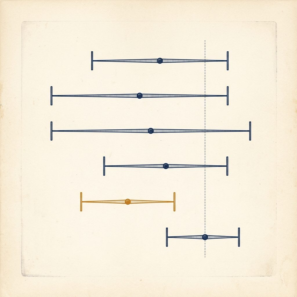
A 1.2-Point Gain, Examined

Your model scores 78.0% on your team's 500-question benchmark. A new checkpoint comes back at 79.2%. Merge it?

Here is the arithmetic the dashboard leaves out. A score of 78% on 500 questions has a standard error of $\sqrt{0.78 \times 0.22 / 500} \approx 1.85$ percentage points. The 95% confidence interval is $\pm 1.96 \times 1.85 \approx \pm 3.6$ pp: the benchmark is telling you the model's true accuracy is somewhere in [74.4%, 81.6%].

The 1.2pp "gain" is a sixth of that interval's width. You know nothing yet.

The Whole Idea in One Formula

A benchmark score is not a property of the model. It is an estimate of how the model would do on the population of questions your benchmark samples from, computed on the $n$ questions you happened to include. Swap in a different draw of questions and the number moves. For a pass/fail metric, the entire machinery fits on one line:

\hat{p} = \frac{k}{n} \qquad \mathrm{SE} = \sqrt{\frac{\hat{p}(1-\hat{p})}{n}} \qquad \mathrm{CI} = \hat{p} \pm z \cdot \mathrm{SE}

where $k$ is the number of questions answered correctly, $n$ is the total, and $z$ sets the confidence level: 1.645 for 90%, 1.96 for 95%, 2.576 for 99%.

Three anchor points to hold onto:

The score you report is $\hat{p}$ , not $p$ . The hat matters. The true accuracy $p$ is invisible; every run of the eval hands you a different $\hat{p}$ in its vicinity.
The bars shrink with $\sqrt{n}$ . Halving the interval costs 4× the questions. This one fact is the entire economics of benchmark size.
$\hat{p}(1-\hat{p})$ peaks at 50%. Scores near the middle are the noisiest; scores near 0% or 100% look precise, and that is exactly where the simple formula starts to lie (more below).

A Worked Example

Your agent solves 156 of 200 tasks.

Point estimate: $\hat{p} = 156/200 = 0.78$ , so you report 78.0%.

Standard error:

\mathrm{SE} = \sqrt{\frac{0.78 \times 0.22}{200}} = \sqrt{0.000858} \approx 0.0293

That's 2.93 percentage points of wobble, built into the eval before anything about the model changes.

95% interval: $78 \pm 1.96 \times 2.93 = 78 \pm 5.74$ , giving [72.3%, 83.7%].

An 11.5-point-wide interval, from a 200-question eval that most teams would call respectable. Any competing model scoring anywhere in that range is statistically indistinguishable from yours.

An Interval That Includes the Impossible

Now the small- $n$ horror story. Your new agent solves 18 of 20 hand-picked hard tasks: 90%. The formula above (called the Wald interval) gives

\mathrm{SE} = \sqrt{\frac{0.9 \times 0.1}{20}} \approx 0.0671 \qquad 90 \pm 1.96 \times 6.71 = 90 \pm 13.15 \; \rightarrow \; [76.8\%,\ 103.2\%]

An interval that includes accuracies your model cannot have. The Wald interval is a normal approximation, and near 0%, near 100%, or at small $n$ , the approximation collapses — it can exceed the axis, and at $\hat{p} = 100\%$ it has zero width, reporting perfect certainty from a handful of questions.

The fix is the Wilson score interval. For 18/20 at 95% it gives a center of 0.8355 and a half-width of 0.1366: [69.9%, 97.2%]. Inside the axis, asymmetric around $\hat{p}$ , and honest about how little 20 questions can tell you. Note it also pulls the center down from 90% — a 90% score on 20 questions is more likely a lucky draw from a weaker model than an unlucky draw from a stronger one.

▶The Wilson formula, with the arithmetic

The Wilson interval recenters the estimate toward 50% and widens correctly near the boundary:

\text{center} = \frac{\hat{p} + z^2/2n}{1 + z^2/n} \qquad \text{half-width} = \frac{z}{1 + z^2/n}\sqrt{\frac{\hat{p}(1-\hat{p})}{n} + \frac{z^2}{4n^2}}

For $k=18$ , $n=20$ , $z=1.96$ (so $z^2 = 3.8416$ ):

$z^2/2n = 3.8416/40 = 0.09604$ , and $1 + z^2/n = 1 + 0.19208 = 1.19208$
center $= (0.9 + 0.09604) / 1.19208 = 0.99604 / 1.19208 = 0.8355$
inside the root: $0.09/20 + 3.8416/1600 = 0.0045 + 0.0024010 = 0.0069010$ , whose square root is $0.08307$
half-width $= (1.96 / 1.19208) \times 0.08307 = 1.6442 \times 0.08307 = 0.1366$

Interval: $0.8355 \pm 0.1366 \rightarrow [0.6990,\ 0.9721]$ , i.e. [69.9%, 97.2%].

My recommendation is to use Wilson always, not just at the extremes: where Wald is fine the two agree to a rounding error, and where they disagree, Wald is the one that's wrong. Brown, Cai and DasGupta (2001) reached the same conclusion after torturing every standard interval; the Wald interval's coverage is erratic even at moderate $n$ and mid-range $p$ .

Ways to Fool Yourself

1. Reading a 1-point leaderboard gap as real. Model A at 71.3%, model B at 70.1%, and the leaderboard sorts A first. On a 300-question eval both scores carry bars of about ±5.2pp. The ranking is a coin flip wearing a medal.

2. "The CIs overlap, so there's no difference." Overlap is not the right test in either direction. Two 95% intervals can overlap while a proper test of the difference still rejects at the 5% level — requiring non-overlap is closer to demanding $z = 2.8$ than 1.96. And if both models answered the same questions, marginal intervals waste most of your information: you should be doing a paired analysis on the per-question deltas, which is the subject of the next post in this series.

3. Trusting Wald near 0%, 100%, or small n. Intervals past 100%, or zero-width intervals proclaiming certainty from 20 questions. Use Wilson.

4. Forgetting what population the interval is about. The CI assumes your questions are a sample from a population you care about. A hand-curated 100-question suite has sampling error plus selection effects that no formula removes. The interval is a floor on your uncertainty, never a ceiling.

5. Twenty subtasks, one guaranteed fluke. Report a dashboard of twenty subtasks with 95% intervals each and you expect one false "regression" per report ( $20 \times 5\%$ ); the chance of at least one is $1 - 0.95^{20} \approx 64\%$ . Either widen the intervals for multiplicity or stop treating every isolated red cell as news.

Try It Yourself

The playground below is a benchmark simulator. You set the model's true accuracy — the number you never get to see in real life — and each press of Run the benchmark draws a fresh $n$ -question eval from it. The current run's interval sits at the top; previous runs stack up beneath it, marked by whether they covered the truth.

True accuracy

78%

current runClick “Run the benchmark” again to stack up intervals.

p̂ (this run)

79.5%

159/200

±2.85pp

√(p̂(1−p̂)/n)

95% CI

[73.9, 85.1]

percent

Width

11.2pp

±5.6pp

0 of 1 run missed the truth5% designed

Experiments to try:

"The vibes benchmark" — 25 questions at 75% true accuracy. Run it a few times and watch the score swing by double digits between runs of the same model.
"Wald meltdown" — keep running until a 24/25 or 25/25 sample pushes the Wald interval past 100%, then flip the method toggle and watch Wilson stay on the axis.
"Coverage check" — 90% intervals. Press ×10 a few times: the tally should settle near 1 miss in 10. That long-run promise is the entire meaning of "confidence."
"Leaderboard reality" → "The workhorse" — same model, 16× the questions, bars exactly 4× narrower. The $\sqrt{n}$ law, live.

Your Turn

The worked example above was mine; this one is yours. Each problem generates a fresh eval result, and the four steps walk from the headline number to the price of improving it. If you get stuck, help escalates gently — a nudge first, then the setup with your numbers plugged in, and only then the full answer.

Practice problem

Retrieval QA

Your model got 222 of 250 retrieval questions right. One score, four questions: the estimate, its wobble, its interval, and the price of shrinking it.

222

answered correctly

250

questions total

accuracy ± error bars

Step 1 of 40/4

The point estimate

The headline number: what accuracy does this run report?

p̂

Field Notes: Error Bars in the Wild

Half-widths of 95% intervals for a model scoring around 70%, on benchmarks people quote daily:

Benchmark	Questions ( $n$ )	95% half-width at $\hat{p} = 0.7$
HumanEval	164	±7.0pp
GPQA-Diamond	198	±6.4pp
GSM8K (test)	1,319	±2.5pp
MMLU (test)	14,042	±0.76pp

A two-point HumanEval gap between two models is deep inside the noise. Much of the day-to-day "model X beats model Y by 2 points" discourse happens entirely inside the bars.

The definitive treatment of this subject is Miller (2024), "Adding Error Bars to Evals" (arXiv:2411.00640), which this series is an attempt to operationalize. Its core moves:

Treat eval questions as drawn from an underlying population, and the score as an estimate of performance on that population.
Compute standard errors from question-level scores via the Central Limit Theorem — which also handles partial-credit and averaged metrics, not just pass/fail.
Report the error bars everywhere: leaderboards, papers, internal dashboards, model cards.
Prefer paired comparisons when two models answer the same questions (next post).
Cluster standard errors when questions come in related groups — multiple questions per document or per scenario are not independent draws (later in this series).

This post is part 1: the unpaired, single-score case. What to report, in one sentence: the sample size, the score, and a Wilson interval — "78.0% on $n = 200$ , 95% CI [71.8%, 83.2%] (Wilson)." Anyone who then asks whether 79.2% "beats" it can be handed the interval.

Code

▶Wilson interval in Python

import math
 
def wilson_ci(k: int, n: int, z: float = 1.96) -> tuple[float, float]:
    """Wilson score interval for k successes in n trials."""
    p = k / n
    denom = 1 + z**2 / n
    center = (p + z**2 / (2 * n)) / denom
    half = (z / denom) * math.sqrt(p * (1 - p) / n + z**2 / (4 * n**2))
    return center - half, center + half
 
print(wilson_ci(156, 200))  # (0.718, 0.832)
print(wilson_ci(18, 20))    # (0.699, 0.972) — compare Wald's (0.768, 1.031)

Or, already implemented and tested: statsmodels.stats.proportion.proportion_confint(k, n, method="wilson").

▶Bootstrap CI for non-binary metrics

When the per-question metric isn't 0/1 — partial credit, BLEU, judge scores on a rubric — the binomial formula doesn't apply, but the resampling version of the same idea does:

import numpy as np
 
def bootstrap_ci(scores, n_boot: int = 10_000, level: float = 0.95, seed: int = 0):
    """Percentile bootstrap CI for the mean of any per-question metric."""
    rng = np.random.default_rng(seed)
    scores = np.asarray(scores)
    idx = rng.integers(0, len(scores), size=(n_boot, len(scores)))
    means = scores[idx].mean(axis=1)
    alpha = (1 - level) / 2
    return np.quantile(means, [alpha, 1 - alpha])

Resample the questions with replacement, recompute the mean each time, take percentiles. For plain accuracy this converges to the intervals above; its value is that it keeps working when your metric doesn't look like a coin flip.