Paired Deltas: Compare Models on the Questions They Share

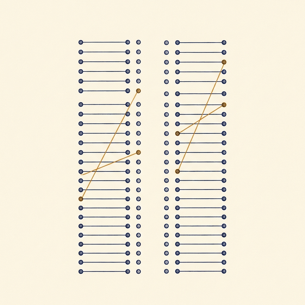
The Two-Point Gap That Wasn't (Yet)

Model A scores 390/500 on your benchmark: 78%. Model B scores 400/500: 80%. Two points. Ship B?

Run the arithmetic from the previous post and it looks hopeless. Treating the two scores as independent measurements:

The 2pp gap is 0.8 standard errors. Indistinguishable from noise. Case closed?

Not quite. Both models answered the same 500 questions, and the score table decomposes:

• Both right: 375
• Both wrong: 85
• B right, A wrong: 25
• A right, B wrong: 15

The 375 questions both models solved tell you nothing about which is better. Neither do the 85 both flubbed. Only the 40 discordant questions carry any information about the difference, and there B won 25 to 15.

Analyze it paired and the picture sharpens: $\Delta = (25 - 15)/500 = 2.0$pp with

Same data. Half the error bar. For free. That is the entire post; the rest is knowing exactly why it works and when it doesn't.

The Whole Idea in One Formula

Score each question $i$ with a per-question difference:

A question both models get right (or both wrong) scores $d_i = 0$. Then the comparison is just a one-sample problem on the $d_i$:

For binary outcomes this collapses to counts. With $b$ = questions only A got right and $c$ = questions only B got right:

The equivalent framing explains where the win comes from. The variance of a difference is

The unpaired analysis assumes the covariance is zero. But two models grading the same questions succeed and fail together: easy questions help both, cursed questions sink both. That shared fate is positive covariance, and pairing subtracts it. Two anchor points:

• Models that agree a lot → big covariance → big win from pairing. Checkpoints of the same run, prompt variants, models from the same family.
• Near-independent models → almost no covariance → pairing subtracts almost nothing. It never hurts; there's just nothing to win.

A Worked Example

The hook's numbers, walked at hand-calculator speed. These are the same four steps the practice exercise below will ask of you.

Step 1: Sort the table

Cross-tabulate the 500 questions by who got them right:

So $a = 375$ (both right), $b = 15$ (A only), $c = 25$ (B only), $d = 85$ (both wrong). The marginals recover the headline scores: A right on $375 + 15 = 390$, B right on $375 + 25 = 400$. The 460 concordant questions just left the conversation; the effective sample is the $b + c = 40$ discordant ones.

Step 2: The delta

Exactly 80% minus 78%, computed the long way. The point of the table isn't the delta, it's the error bar.

Step 3: The error bar, twice

Unpaired, from the hook: $\sqrt{1.85^2 + 1.79^2} = 2.58$pp.

Paired, from the discordant counts:

Same table, and the error bar shrank by a factor of $2.58 / 1.26 = 2.04$. To buy that shrink with sample size instead, you'd need roughly four times as many questions.

Step 4: The interval and the call

Honest conclusion: the interval still crosses zero. Pairing halved the bars and the verdict is still "promising, not proven." A significance test agrees: under the null hypothesis that neither model is better, each discordant question is a fair coin flip, so B's 25 wins out of 40 follow $\mathrm{Binomial}(40, 0.5)$. The two-sided exact p-value is 0.154. That's McNemar's test, and $p \approx 0.15$ is not a green light.

This is worth sitting with: pairing is not a machine for manufacturing significance. It removes noise you never had to accept, and then the data says whatever it says.

Ways to Fool Yourself

1. "The two confidence intervals overlap, so there's no difference." The classic. A's CI is [74.4, 81.6] and B's is [76.5, 83.5]; they overlap generously, and none of that matters. Overlap of individual CIs is not the test. The test is whether the CI on the delta excludes zero, and with positive covariance the delta's CI can be far tighter than the overlap picture suggests.

2. Comparing scores from different question subsets or benchmark versions. If A ran on v1.2 of the benchmark and B on v1.3, there is no pairing to exploit, and it's worse than that: the question-mix difference is a confound baked directly into the delta. Rerun on identical questions before comparing at all.

3. Keeping only the aggregate scores. If your eval harness logs "78.0%" and discards per-question outcomes, you paid for the pairing and then deleted it. The 2×2 table cannot be reconstructed from two percentages, and neither can the paired error bar.

4. Running the paired test on 20 slices and reporting the one that hit. Paired tests are still tests. Slice by topic, language, difficulty, and format, and at $\alpha = 0.05$ one slice in twenty clears the bar by luck. Decide the slices in advance, or correct for the shopping trip.

5. Expecting pairing to rescue a comparison between strangers. The win scales with agreement. Two models with near-independent errors have nothing for pairing to subtract, and the paired bar will sit almost exactly on top of the unpaired one. The playground's "Strangers" preset makes this painfully concrete.

Try It Yourself

Two simulated models answer the same $n$ questions. You control the true accuracy gap and how correlated the models' per-question outcomes are; both analyses are then computed from the same simulated table.

Experiments to try:

• "Twins" (ρ = 0.8, Δ = +2pp) — the paired bar is roughly half the unpaired one. At n = 500 the pairing alone often decides the verdict.
• "Strangers" (ρ = 0, Δ = +2pp) — the two bars nearly coincide. No shared covariance, nothing to subtract.
• "Dead heat" (Δ = 0, ρ = 0.6) — reshuffle a few times and watch $\hat{\Delta}$ wobble around zero. Any run where an interval clears zero is your one-in-twenty false alarm in the wild.
• "Real jump" (Δ = +4pp, ρ = 0.6) — even the unpaired analysis usually catches this at n = 500. Now drag n down and find the range where only the paired analysis does.
• Fix everything and sweep ρ from 0 to 0.9: exactly one of the two bars moves. The unpaired analysis literally cannot see the correlation.

Your Turn

Twelve items, two systems, one honest interval. Each problem generates a fresh table in a new setting, and the four steps mirror the walkthrough exactly. If you get stuck, help escalates gently: a nudge first, then the setup with your numbers plugged in, and only then the full answer.

Field Notes

Use a paired delta any time two systems answered the same items: two checkpoints, two prompts, two RAG configurations, two judge rubrics scored against the same key. Report three things: $\Delta$, its paired 95% CI, and the discordant counts $b$ and $c$. The counts cost you one sentence and let any reader re-derive the rest.

This is not exotic advice. Miller (2024, arXiv:2411.00640) makes paired differences the explicitly recommended analysis for model comparisons in "Adding Error Bars to Evals," for exactly the covariance reasons above. Dietterich (1998) reached the matching conclusion for classical classifiers: among the tests he benchmarked for comparing two learners on one test set, McNemar's test was one of the few with acceptable Type I error. The test itself is from McNemar (1947); the eval-harness use case is new, the statistics are not.

In practice:

• Persist per-item outcomes. A per-question correctness log is the difference between a paired analysis and an apology. Aggregate scores are a lossy compression you can compute later; the reverse direction doesn't exist.
• Run both models on identical question versions. Same prompts, same few-shot examples, same scoring script. Any version skew turns into fake delta.
• Bootstrap paired, by resampling items. When the statistic is gnarlier than mean accuracy (pass@k, judge scores, length-normalized anything), resample items with replacement and keep each item's pair of outcomes together. Resampling models independently silently rebuilds the unpaired analysis.

import numpy as np
 
def paired_bootstrap_ci(a, b, reps=10_000, seed=0):
    """a, b: per-item outcomes for models A and B, aligned by item."""
    rng = np.random.default_rng(seed)
    n = len(a)
    deltas = np.empty(reps)
    for r in range(reps):
        idx = rng.integers(0, n, n)   # resample ITEMS; pairs stay together
        deltas[r] = b[idx].mean() - a[idx].mean()
    return np.percentile(deltas, [2.5, 97.5])

Where this sits in the series: the previous post put an error bar on a single score, this one compares two scores, and the next one handles questions that arrive in correlated clusters, which quietly breaks the $\sqrt{n}$ in everything above.

Code

import numpy as np
from scipy import stats
 
def paired_delta(a: np.ndarray, b: np.ndarray):
    """Paired delta and 95% CI from two aligned boolean arrays."""
    d = b.astype(float) - a.astype(float)   # per-question difference in {-1, 0, +1}
    n = len(d)
    delta = d.mean()
    se = d.std(ddof=1) / np.sqrt(n)
    return delta, se, (delta - 1.96 * se, delta + 1.96 * se)
 
def mcnemar_exact(a: np.ndarray, b: np.ndarray) -> float:
    """Two-sided exact McNemar p-value: discordant wins vs Binomial(b+c, 0.5)."""
    b_only = int((a & ~b).sum())    # A right, B wrong
    c_only = int((~a & b).sum())    # B right, A wrong
    return stats.binomtest(c_only, b_only + c_only, 0.5).pvalue
 
a = np.array([...], dtype=bool)   # model A correct, one entry per question
b = np.array([...], dtype=bool)   # model B correct, same question order
 
delta, se, ci = paired_delta(a, b)
print(f"delta = {delta:+.4f}, SE = {se:.4f}, 95% CI = [{ci[0]:.4f}, {ci[1]:.4f}]")
print(f"McNemar exact p = {mcnemar_exact(a, b):.4f}")

Further Reading

• Miller, E. (2024). "Adding Error Bars to Evals: A Statistical Approach to Language Model Evaluations." arXiv:2411.00640
• Dietterich, T. G. (1998). "Approximate Statistical Tests for Comparing Supervised Classification Learning Algorithms." Neural Computation 10(7), 1895–1923.
• McNemar, Q. (1947). "Note on the sampling error of the difference between correlated proportions or percentages." Psychometrika 12(2), 153–157.