Correlation Is Not Calibration

The Judge That Passed the Wrong Test

You want an LLM judge to replace your human graders, so you run the validation study everyone runs: 200 responses, each scored 1–10 by a human expert and by the judge. The result comes back Pearson r = 0.91. Ship it?

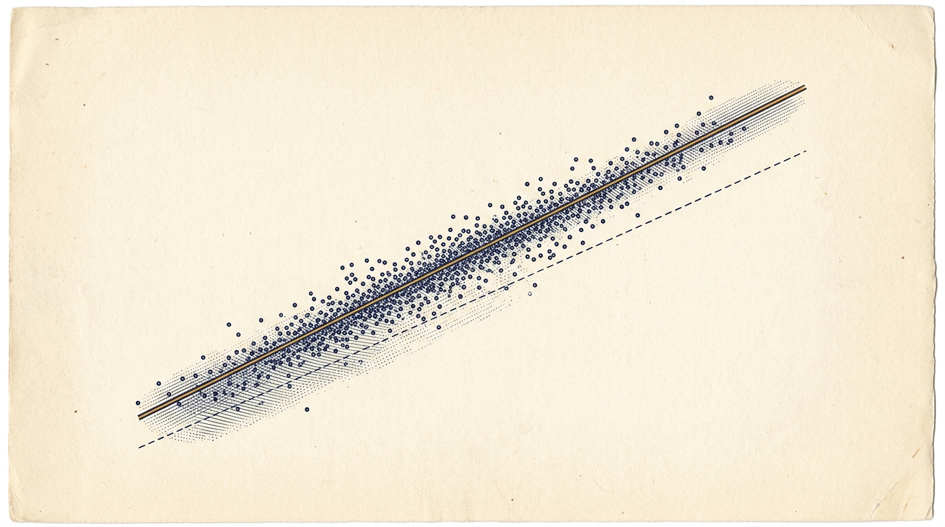
Look at the raw scores first. On those same 200 responses the humans averaged 5.8; the judge averaged 7.3. The judge scores everything about a point and a half higher, and r is structurally incapable of noticing. Pearson correlation is invariant to shifting and scaling: add 1.5 to every judge score, or double them all, and r does not move. A judge can rank responses perfectly and still grade on its own private curve.

That matters the moment your pipeline consumes scores rather than orderings: an "auto-approve at 8" threshold, a dashboard comparing this month's judge to last month's, a comparison across two judges with different curves. For all of those, r = 0.91 is answering a different question than the one you asked.

The Whole Idea in One Formula

r = \frac{\sum_i (x_i - \bar{x})(y_i - \bar{y})}{\sqrt{\sum_i (x_i - \bar{x})^2 \, \sum_i (y_i - \bar{y})^2}}

The numerator asks whether $x$ and $y$ move together around their own means; the denominator divides out each rater's spread. An equivalent reading: standardize both raters and take the average product,

r = \frac{1}{n}\sum_i z_{x_i} \, z_{y_i}

$r = 1$ : the points sit exactly on an upward-sloping line — any upward slope, any intercept
$r = 0$ : no linear relationship
$r = -1$ : exactly on a downward-sloping line

The z-scoring is where both the feature and the bug live. Subtracting each rater's mean and dividing by each rater's spread makes r unit-free — you can correlate meters with dollars. It also means r deletes exactly two facts before it looks at anything: where each rater's scale sits, and how wide it is. Those two facts are calibration. Formally, for any constant $a$ and any $b > 0$ ,

r(x,\ a + b\,y) = r(x,\ y)

Feature and bug, same theorem.

A Worked Example

Five responses, scored by a human ( $x$ ) and a judge ( $y$ ):

Response	Human ( $x$ )	Judge ( $y$ )
1	2	4
2	4	5
3	5	6
4	6	7
5	8	9

Step 1: Means

$\bar{x} = \frac{2+4+5+6+8}{5} = 5$ , and $\bar{y} = \frac{4+5+6+7+9}{5} = 6.2$ .

Step 2: Deviations and their products

Response	$x_i - \bar{x}$	$y_i - \bar{y}$	Product
1	$-3$	$-2.2$	$6.6$
2	$-1$	$-1.2$	$1.2$
3	$0$	$-0.2$	$0.0$
4	$1$	$0.8$	$0.8$
5	$3$	$2.8$	$8.4$

Sum of products: $6.6 + 1.2 + 0 + 0.8 + 8.4 = 17$ .

Squared deviations: $\sum (x_i-\bar{x})^2 = 9+1+0+1+9 = 20$ and $\sum (y_i-\bar{y})^2 = 4.84+1.44+0.04+0.64+7.84 = 14.8$ .

Step 3: Pearson r

r = \frac{17}{\sqrt{20 \times 14.8}} = \frac{17}{\sqrt{296}} \approx \frac{17}{17.205} \approx 0.988

Nearly perfect. Now the rank version.

Step 4: Spearman ρ

Both raters put the five responses in the same order, so the ranks are 1–5 against 1–5, every rank difference $d_i = 0$ , and $\sum d_i^2 = 0$ :

\rho = 1 - \frac{6 \times 0}{5(5^2 - 1)} = 1 - \frac{0}{120} = 1

Exactly 1. The ordering is flawless.

Step 5: The number neither of them saw

\bar{y} - \bar{x} = 6.2 - 5 = +1.2

ρ says the ordering is perfect, r says nearly-linear, and neither noticed that the judge adds 1.2 points to everything. Concretely: under an "auto-approve at 6" rule, response 3 gets approved by the judge and rejected by the human — on a dataset where $r = 0.988$ and $\rho = 1$ .

Spearman: Correlation on Ranks

Spearman's ρ is nothing exotic — it is Pearson's r computed on the ranks instead of the scores. When there are no ties, the arithmetic collapses to a shortcut:

\rho = 1 - \frac{6\sum_i d_i^2}{n(n^2 - 1)}

where $d_i$ is the difference between the two ranks for item $i$ . For $n = 5$ the denominator is $5 \times 24 = 120$ , and $\sum d_i^2$ runs from 0 (identical orderings, $\rho = 1$ ) to 40 (a perfect reversal, $\rho = 1 - 240/120 = -1$ ).

Ranks buy you two kinds of robustness. A wild outlier can only move to the end of the rank order — it cannot drag the whole line toward itself the way it drags r. And any relationship that is monotone but nonlinear (a judge that compresses the top of the scale, say) keeps $\rho$ high while r sags. The cost is that ρ is even more forgetful than r: it discards not just location and scale but the sizes of all the gaps. Two judges who order 100 responses identically get $\rho = 1$ even if one scores everything 5.0–5.4 and the other 1–10.

Ways to Fool Yourself

1. Reading r as calibration. The theme of this post. Both r and ρ are pure association measures; a +1.5-point systematic shift is mathematically invisible to them. If any downstream decision consumes the scores themselves, you must also report the shift.

2. Range restriction. Validate the judge only on strong responses and r collapses — for a good judge. A faithful judge with per-item noise $\sigma = 0.8$ scores about r ≈ 0.96 across the full 1–10 range, but restrict the validation set to responses humans scored 7 or above and the same judge drops to r ≈ 0.73. Nothing about the judge changed; you shrank the signal variance and kept the noise. Curated "high-quality eval sets" do this to themselves constantly.

3. A single outlier can buy you 0.2 of Pearson r (or more). In one simulation: twenty mid-scale pairs with r = 0.29 and ρ = 0.32. Append a single pair at (10, 10) — one response that is obviously brilliant to both raters — and r jumps to 0.63 while ρ crawls to 0.41. If your validation set includes a couple of unambiguous disasters and masterpieces, they can carry the entire correlation while the mid-pack, where all the real grading decisions live, contributes nothing.

4. Likert ties and the shortcut formula. Integer scales produce ties — lots of them on a 1–5 scale, plenty on 1–10. The $1 - 6\sum d^2 / n(n^2-1)$ shortcut assumes ties don't exist and quietly returns the wrong number when they do. Use the tie-aware version: assign tied values the average of the rank positions they span ("midranks"), then compute Pearson on the ranks. That is what scipy.stats.spearmanr does; the shortcut is for hand arithmetic on tie-free data, like the exercise below.

5. Aggregate r can hide per-slice miscalibration. Suppose the judge runs +1.1 points hot on code answers and −0.9 cold on prose. Pooled, the mean bias is roughly zero and r looks healthy — the two slices cancel in the aggregate, Simpson-style. Every per-slice decision (routing, thresholds, model comparisons within a category) is still wrong in both directions. Slice before you celebrate.

Try It Yourself

The playground simulates a judge with three dials — a systematic shift (bias), a scale-use factor (slope), and per-item noise — against humans spread across the full 1–10 range. Watch which of the four tiles move when you turn each dial.

Bias+0.0

Slope1.00

Noise σ0.8

Items160

Pearson r

0.95

Spearman ρ

0.95

Mean bias

−0.08

MAE

0.64

Experiments to try:

"Faithful judge" — the baseline: r ≈ 0.95, ρ right behind it, bias ≈ 0. Now drag Bias to +2 and watch r and ρ stand perfectly still while mean bias and MAE jump. That's the invariance theorem, live.
"Grade inflator" — the whole cloud floats above the judge = human line. Every ranking number stays flattering; only the calibration tiles complain.
"Compressor" — slope 0.4 maps the humans' 1–10 onto roughly 4–7. r stays high because compression is linear; look at how flat the cloud is against the reference line. An 8 from this judge means almost nothing.
"Noise machine" — r collapses. No recalibration fixes a judge that can't rank; the fix is a better judge, not a better offset.
Drop Items to 20 and press Reshuffle a few times. Correlations on small validation sets bounce hard — a preview of why the error-bars strand of this series exists.

Your Turn

The worked example above was mine; these are yours. Each problem deals out five fresh scores from two raters, and the four steps mirror the walkthrough: ranks, Σd², ρ, then the bias ρ never saw. If you get stuck, help escalates gently — a nudge first, then the setup with your numbers plugged in, and only then the full answer.

Practice problem

LLM Judge Validation

The human expert and the LLM judge each scored 5 chatbot responses from 1–10. Rows are sorted by the human expert's score, so the human ranks are done for you. Work down to ρ — then find the number it missed.

Response	Human score	Human rank	Judge score	Judge rank
#1	2	1	5	–
#2	3	2	6	–
#3	4	3	4	–
#4	8	4	9	–
#5	10	5	10	–

Step 1 of 40/4

Rank the judge

Rank the LLM judge's scores from 1 (lowest) to 5 (highest), one rank per chatbot response.

#1 (Judge 5)

#2 (Judge 6)

#3 (Judge 4)

#4 (Judge 9)

#5 (Judge 10)

Field Notes: What a Judge Validation Report Needs

A single correlation is not a validation. A defensible judge report has four parts:

1. Ranking power. Spearman's ρ (or Kendall's τ, which counts concordant vs. discordant pairs and behaves better on small tied samples). This answers: can the judge order responses the way humans do?

2. Calibration. Mean bias (judge − human, signed), MAE, and a look at how the differences behave across the score range — plot judge − human against the human score, Bland–Altman style. Bland & Altman (1986) made exactly this argument to medical researchers comparing measurement methods: correlation measures association, not agreement, and two instruments can correlate at 0.99 while disagreeing by a clinically fatal constant. Method-comparison studies dropped r for difference plots four decades ago; judge validation reports can too.

3. Chance-corrected categorical agreement. If the scores get bucketed downstream — accept/reject, severity bands — report agreement on the buckets corrected for chance: Krippendorff's alpha or Cohen's kappa. Raw bucket agreement inherits every base-rate illusion covered earlier in this series.

4. Slice-level checks. Repeat 1–3 per category (code vs. prose, short vs. long, topic areas). This is where the known LLM-judge failure modes surface. Zheng et al. (2023), the MT-Bench and Chatbot Arena paper, measured three of them directly: position bias (GPT-4 favored the first-presented answer in pairwise comparisons), verbosity bias (judges rewarded longer answers, failing their "repetitive list" attack in most tested cases), and self-enhancement bias (some judges rated their own model family's outputs higher). None of these show up in an aggregate r against humans on a balanced set; all of them show up in sliced calibration checks.

One pragmatic dodge deserves a mention: pairwise-preference judging ("which response is better, A or B?") sidesteps calibration entirely. No scores, no scale, nothing to drift — part of why Chatbot Arena is built on it. But it does not sidestep the biases above: position bias and verbosity bias were measured in that pairwise setting. Preference judging trades the calibration problem for a counterbalancing problem (swap the order and judge twice).

Code

▶Python: the whole validation in six lines

import numpy as np
from scipy.stats import pearsonr, spearmanr
 
human = np.array([2, 4, 5, 6, 8])
judge = np.array([4, 5, 6, 7, 9])
 
r, _ = pearsonr(human, judge)
rho, _ = spearmanr(human, judge)     # tie-aware: uses average ranks (midranks)
bias = float(np.mean(judge - human)) # the number r can't see
mae = float(np.mean(np.abs(judge - human)))
 
print(f"r={r:.3f}  rho={rho:.3f}  bias={bias:+.2f}  mae={mae:.2f}")
# r=0.988  rho=1.000  bias=+1.20  mae=1.20

spearmanr handles ties with average ranks, so it is safe for Likert-style integer scores. Do not use the $1 - 6\sum d^2/n(n^2-1)$ shortcut on tied data.

▶R

cor(human, judge, method = "pearson")
cor(human, judge, method = "spearman")  # midranks for ties
mean(judge - human)                     # calibration, one line